Unlocking Efficiency: The Importance of Predictive Maintenance
Explore how predictive maintenance powered by AI is transforming industries like mining and manufacturing by reducing costs and minimizing downtime.
Apr 23, 2025 · Lukas Wiku, Vincentius C. Calvin
Understanding Machine Failure
Machine failure is a critical event which occurs when a machine or one of its components can no longer perform within its intended operational parameters. These parameters—known as performance thresholds—are usually defined by manufacturers based on engineering tolerances, historical assumptions, and safety margins. In real-world applications, however, these thresholds can vary widely depending on the underlying operating conditions, usage patterns, and even enviromental stresses.
Traditionally, failure has been thought of as a linear process—declining over time. However, a foundational study by Nowlan and Heap disrupted this notion. Their findings revealed that the majority of failures occur randomly and are not directly related to the age of the equipment iself. In fact, only a small percentage of failures folllowed a clear wear-out pattern. This discovery marked a turning point in maintenance philosophy and laid the initial groundowrk for condition-based and predictive maintenance approaches.
To visualize these failure trends, the Bathtub Curve is widely referenced:
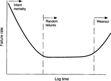
source: https://www.sciencedirect.com/topics/engineering/bathtub-curve
The curve gets its name from its shape and consists of three distinct failure regions:
-
Infant Mortality Phase: This early phase is characterized by a high rate of failures shortly after deployment. These failures are often the result of manufacturing defects, installation errors, or early design flaws. Quality control and burn-in testing are common practices to mitigate this risk.
-
Normal Life Phase: Once early defects are resolved, the equipment enters a stable operational period. In this phase, the failure rate is relatively low and consistent—but importantly, most of the failures that do occur here are random and unpredictable. They may be triggered by anomalies in usage, environmental fluctuations, or unforeseen stresses.
-
Wear-Out Phase: As the machine ages, components begin to degrade due to fatigue, corrosion, or material breakdown. The failure rate increases gradually, and this stage marks the traditional concept of aging-related failure that preventive maintenance programs were originally designed to address.
While the Bathtub Curve itself is a simplification and does not represent all asset types equally (especially modern digital or software-integrated systems), it provides a useful mental model. More importantly, it provides us with a key hypothesis to begin with: only a fraction of failures are truly time-dependent. The rest require a deeper understanding of real-time operating conditions, usage variability, and anomaly detection.
This insight challenges organizations to rethink maintenance from being strictly time-based to being data-informed and condition-aware. As we’ll explore further, this shift is not just a technical evolution—but a strategic business imperative.
Maintenance Strategies
To manage the risk of machine failure and ensure operational continuity, organizations implement various maintenance strategies. These strategies have evolved over time—from simple reactive fixes to sophisticated predictive systems driven by data and AI.
Each approach carries trade-offs in terms of cost, risk, and efficiency. Understanding each of these approaches would be undoubtedly crucial, especially for industries where downtimes directly impacts revenue, safety, and repuation—all being equally crucial.
-
Reactive Maintenance (Run-to-Failure)
Reactive maintenance is the most basic form—equipment is used until it breaks, at which point repairs or replacements are made accordingly.
This approach may seem cost-effective in the short term, especially for non-critical assets where failure doesn't lead to major disruption. However, for most enterprise environments, waiting for failure is a high-stakes gamble.
- Pros: No upfront planning or monitoring required.
- Cons: Unplanned downtime, higher repair costs, potential safety hazards, and production losses.
Example: In a manufacturing plant, allowing a conveyor belt motor to fail during production without any prior warning would halt an entire production line, causing cascading delays and missed delivery deadlines.
-
Preventive Maintenance (Scheduled Intervals)
Preventive maintenance schedules inspections, servicing, or part replacements based on fixed time or usage intervals—such as operating hours, mileage, or calendar dates.
It is widely used and often mandated by equipment manufacturers. However, it is often based on historical averages, not on the actual condition of the asset.
- Pros: Reduces catastrophic failures, follows manufacturer guidelines, easier to manage at scale.
- Cons: May result in unnecessary maintenance for lightly used assets, or insufficient intervention for heavily used ones.
Example: A fleet of delivery trucks may be serviced every 10,000 km. However, it is logical to assume that a specific truck operating in hilly terrain may degrade faster than another used on flat roads—despite having traveled the same distance. Without adapting to real-world usage, preventive maintenance can either overspend on maintenance or fail to prevent issues altogether.
-
Predictive Maintenance (Data-Driven, Condition-Based)
As opposed to the previous two, predictive maintenance leverages real-time data from sensors embedded in machinery—capturing metrics such as temperature, vibration, oil quality, pressure, and acoustic signals. The data streams are then analyzed using AI and machine learning algorithms to estimate the Remaining Useful Life (RUL) of components.
This approach enables "just-in-time" maintenance—intervening only when the system detects that failure is likely within a specific window.
- Pros: Reduces unplanned downtime, extends asset life, lowers operational and labor costs, improves safety and reliability.
- Cons: Requires investment in sensors, data infrastructure, and model development.
Example: In a power plan, vibration data from turbine bearings can indicate the onset of imbalance or misalignment. With predictive models, engineers can plan a controlled shutdown before failure occurs—minimizing repair costs and preventing energy service disruption.
Why the Shift to Predictive Matters
Modern operational environments are far more complex and fast-paced than when time-based maintenance models were developed. Factors such as increased asset complexity, rising energy and labor costs, and tighter delivery SLAs demand smarter, leaner, and more adaptive maintenance models.
Predictive maintenance offers a transformative leap by enabling enterprises to:
- Reduce maintenance costs by avoiding unnecessary service.
- Prevent revenue loss from unexpected downtime.
- Increase the overall lifespan and availability of critical assets.
- Align maintenance planning with business operations and inventory management.
In short, predictive maintenance is no longer a nice-to-have—it is a competitive advantage.
Bridging Into Real-World Application
While the strategic benefits of predictive maintenance are clear, its true value becomes even more apparent when applied to real-world scenarios. In practice, the limitations of preventive maintenance are especially visible in industries where machinery operates under unpredictable, variable conditions.
Take, for example, heavy equipment manufacturers like Komatsu. They provide scheduled service recommendations—after 500, 1,000, 2,000, and 6,000 hours of operation. These intervals are designed based on typical fatigue models and average usage assumptions. But in reality, machine performance rarely adheres to “average.”
- Under intense workloads or harsh environments, a machine might fail well before its recommended service interval.
- Conversely, in lighter-duty applications, machines can operate safely beyond those checkpoints—making scheduled maintenance unnecessary and costly.
This mismatch reveals the core flaw of time-based servicing: it lacks visibility into the actual condition of the equipment. It treats all use cases equally, regardless of how differently machines are stressed and utilized.
A smarter approach involves continuously assessing the real-time condition of machinery to understand how long it can safely operate before intervention is truly needed. By identifying early warning signs of degradation—through vibration patterns, temperature changes, or pressure fluctuations—maintenance can be scheduled precisely when it’s required, avoiding both premature service and catastrophic failure.
This philosophy forms the foundation of predictive maintenance, and it’s more than theory—it’s testable.
From Theory to Practice: Experimenting with Predictive Maintenance
To illustrate the difference in outcomes between preventive and predictive maintenance, we’ll turn to a practical dataset: the NASA Turbojet Engine Dataset. This dataset captures sensor readings over time from simulated jet engines, tracking their performance as they gradually degrade toward failure.
By comparing predictive models trained on these sensor patterns against traditional scheduled maintenance assumptions, we can later quantify the economic and operational value of predictive strategies in action.
Importing modules
For this experiment, we’ll use Python with standard libraries for data processing and machine learning:
Dataset Exploration
Each row in the dataset represents a snapshot of an engine’s state at a given time cycle. The columns are structured as follows:
- unit_number: Identifier for each engine (1–100)
- time_cycles: The cycle count (i.e., usage time step) for the engine
- setting_1 to setting_3: Operational settings, which may affect degradation
- s_1 to s_21: Sensor readings that reflect internal physical conditions like temperature, pressure, and vibration
We start by naming the columns for better readability:
The objective
Our goal is to estimate how many cycles an engine can continue operating before it reaches the end of its useful life. In other words, based on its current usage (number of completed cycles) and condition (captured by sensor readings), we aim to predict the remaining useful life (RUL) of each engine.
Typically, engines degrade over time, which is reflected in factors such as increased oil temperature, decreased thrust, and so on. The acceptable threshold for degradation can vary depending on operational context and user requirements.
A quick look on the training set
Looking at the dataset, it's clear that this is time series data. Each row represents a snapshot in time for a particular engine. The unit_number resets after a sequence of time_cycles, indicating data for a new engine unit.
To better understand engine lifespans, we can group the data by unit_number and look at the maximum cycle each engine reached before failure:
It’s not immediately obvious how each sensor reading relates to the engine’s remaining life. To explore this relationship, we’ll use unit_number == 1 as an example and visualize how sensor values evolve throughout its lifetime.
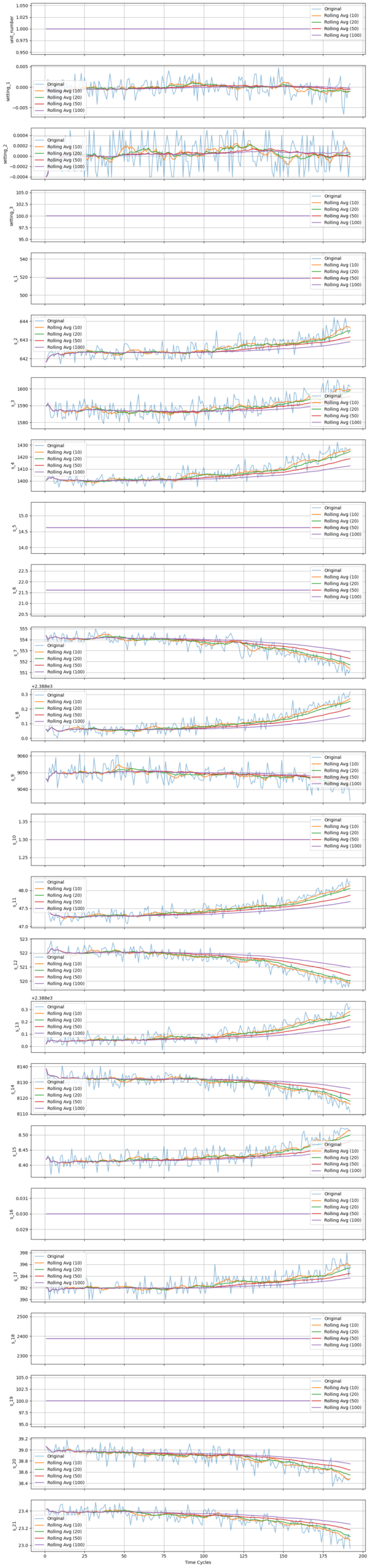
Data Insights & Observations
Looking at the plots, we can intuitively see that some sensors change over time, while others remain static. This suggests that certain sensors correlate with the engine's age or its Remaining Useful Life (RUL). In fact, RUL is a standard metric used to determine "how old" or "how used" an engine is.
Keep in mind that RUL is a key concept in predictive maintenance and will be referenced frequently throughout this article.
As RUL is not directly provided in the dataset — we’ll need to calculate it ourselves.
Preprocessing
1. Calculating RUL
Given that column 2 (time_cycles) represents the current cycle, and the last sensor reading for each unit corresponds to the end of its life, RUL should decrease over time. We can calculate RUL by subtracting the current_cycle from the last_cycle for each engine unit. Here's how to implement this in pandas:
As expected, RUL decreases as time_cycle increases—a logical trend. Our ultimate goal with this dataset is to build a model that can predict RUL. The test_df provides partial engine run data, including cycle counts and sensor readings taken sometime before the end of each engine's life. Our task is to use this information to accurately estimate how many cycles are left before failure occurs.
2. Filtering
Based on the earlier plots, sensors s_1, s_5, s_6, s_10, s_16, s_18, and s_19 appear static — they don’t change over time and likely offer little predictive value. We'll drop them, along with the unit_number, which is no longer needed.
Preparing the dataset
1. Splitting into Training, Validation, and Testing Sets
Now let's prepare our dataset. First, we separate the features (X) and the target (y) from the training set. Then, we split the data into a 70:30 ratio for training and validation.
2. Scaling
Scaling is an important step in machine learning. It helps models learn more effectively by reducing the numerical distances between features, which can otherwise lead to instability or numerical overflow. Moreover, scaling prevents features with larger ranges from dominating the learning process, reducing bias in the model.
Now that the dataset is preprocessed, we’re ready to build some prediction models!
Modeling
This is a multivariate regression problem. Our input features (x1, x2, ..., xi) are the sensor readings, and the target (y) is the RUL. There are many machine learning techniques to solve this type of problem. In this article, we’ll explore and compare three popular models:
- SVM (Support Vector Machine)
- RF (Random Forest)
- GB (Gradient Boosting)
1. Model Initialization
2. Model Fitting
Fit each model using the exact same train set
3. Model Evaluation
Based on these results, the SVR_model performs best in terms of Test RMSE and R², and it generalizes well. In contrast, the Random Forest model appears to overfit the training and validation sets.
With this simple setup, we were able to predict the RUL with an RMSE of 24.03 and R² of 0.66. While these results aren't particularly high, they’re still usable as a baseline. Of course, there are many ways to improve the model's performance — but for this article, this serves as a solid starting point.
Implementation and use cases
So far, we’ve built a reasonably performing model. Next, let’s compare its effectiveness against a preventive maintenance approach.
Currently, we have test_df_y, which contains the ground-truth RUL values. To make a meaningful comparison, we also need to calculate the actual time each engine would fail — i.e., the ground-truth time_cycles at the point of failure.
Preventive maintenance: The naive approach
1. Average End-of-Life Cycle
In this approach, we assume that all engines are identical and should be maintained based on a fixed threshold. Normally, this threshold would be defined by manufacturer guidelines. However, since the dataset is simulated, no such policy is provided.
As a substitute, we can use the average end-of-life cycle (i.e., the average of each engine's final time cycle in the training set) as a reasonable threshold.
Using the average as a maintenance threshold leads to 57 engines being overestimated — meaning they fail before maintenance is performed. In real-world scenarios, these failures could lead to serious operational disruptions or even safety hazards.
To mitigate this risk, a more conservative threshold can be used: the minimum end-of-life cycle observed.
2. Minimum End-of-Life Cycle
To get a better understanding of the impact, let's update our calculate_maintenance function and visualize it!
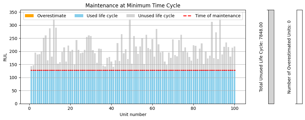
This conservative strategy avoids all failures, ensuring that engines are serviced before their end-of-life. However, this comes at a cost — 7848 total life cycles are wasted due to premature maintenance.
This leads us to a crucial question:
Can we optimize the maintenance timing—extending or postponing it slightly—to make better use of the remaining life cycles and reduce costs, while still avoiding unexpected failures?
Absolutely — and that’s where predictive maintenance shines.
Instead of using a static threshold, predictive maintenance uses model-based predictions to dynamically determine the remaining life for each engine. This enables customized, per-engine thresholds, leading to smarter, safer, and more cost-efficient maintenance schedules.
Predictive Maintenance Approach
The first step is to create a function that calculates a variable end-of-life cycle using the model's predictions:
Unlike previous approaches where the end-of-life cycles were the same for all engines, svr_end_of_cycle provides individualized estimates, accounting for each engine's condition. Let's visualize the result:
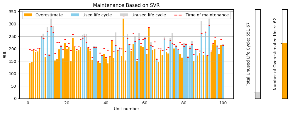
This approach successfully reduced the unused life cycles to just 551.66 cycles, a significant improvement over the previous methods. However, it resulted in 62 engines being overestimated, which is still a safety concern. Unfortunately, this is not what we want, yet.
1. SVR Adjusted by Average
To reduce the risk of overestimating engine RUL, we can introduce a correction constant. This constant adjusts predictions downward based on the average prediction error, calculated only from overestimated cases:
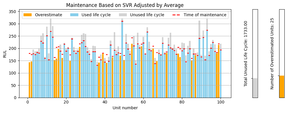
With the average correction applied, the number of overestimated engines decreases. If we would like to be even more conservative, we can adjust the predictions using the minimum observed error instead.
2. SVR Adjusted by Minimum
Using the same adjusting concept, we slightly modify our previous function as follows:
Some predictions drop below the min_test_end_of_cycle, so let’s clip them:
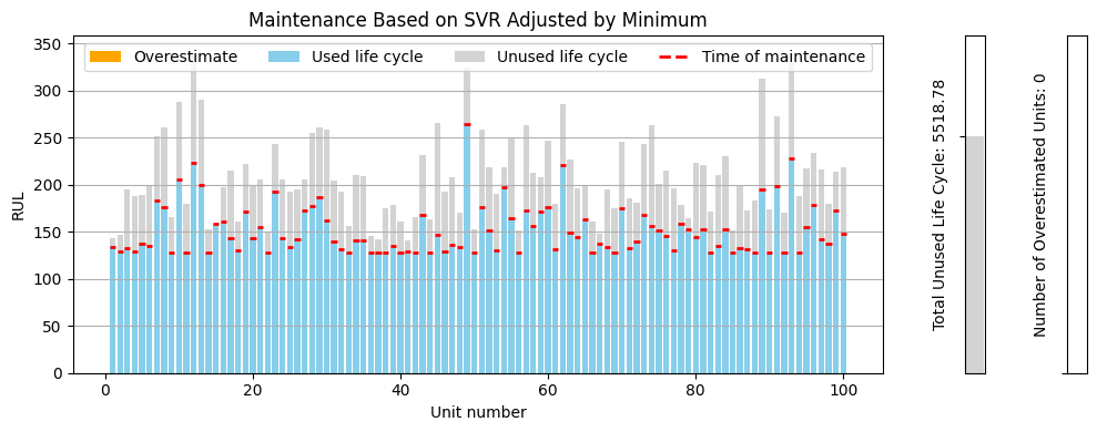
Cost-Benefit Analysis: Predictive vs. Preventive Maintenance
Now that we’ve reduced the number of overestimated engines to zero and reclaimed 2,329.22 unused life cycles, let’s quantify this in terms of real-world savings.
Maintenance Cost Assumption
Let’s assume:
- The cost of a single engine maintenance is $9,000
- Manufacturers typically perform preventive maintenance every 128 cycles
(this was the minimum observed end-of-life cycle across all engines)
This implies a cost per engine cycle:
So, every unused cycle costs approximately $70.31 in wasted maintenance potential.
Savings from Predictive Maintenance
From earlier, we found that:
- The naive preventive maintenance strategy led to 7,848 unused life cycles
- Our optimized predictive approach reduced that to 5,518.78 cycles
- That’s a reduction of 2,329.22 cycles, which would otherwise have been wasted
Let’s calculate the cost savings:
💡 By switching to predictive maintenance, we saved approximately $163,773, just from better timing alone—without requiring more maintenance or hardware changes.
Summary
| Strategy | Unused Life Cycles | Estimated Failures | Total Maintenance Cost Impact |
|---|---|---|---|
| Naive (Minimum Policy) | 7,848 | 0 | Baseline ($0 saved) |
| Predictive (Adjusted) | 5,518.78 | 0 | $163,773 saved |
This example clearly demonstrates how AI-driven predictive maintenance not only preserves equipment health but also delivers significant financial impact—a compelling case for its adoption across asset-heavy industries like aviation, manufacturing, or energy.
Closing Thoughts
In today's competitive and asset-intensive industries, efficiency, reliability, and cost optimization are non-negotiable. Traditional maintenance strategies—especially preventive maintenance based on fixed schedules—often lead to a tradeoff between unexpected breakdowns and premature servicing. Both scenarios come with significant operational and financial costs.
This is where predictive maintenance stands out as a strategic advantage. By harnessing historical sensor data and machine learning models, we can accurately estimate an asset's remaining useful life (RUL) and make informed, real-time decisions on when to service equipment. As demonstrated in our analysis, predictive maintenance significantly reduces unnecessary maintenance while still preventing operational failures—saving thousands of dollars per fleet with every optimization cycle.
More importantly, predictive maintenance isn't just about cost savings. It empowers businesses with:
- Higher equipment uptime and availability
- Extended asset lifecycle and ROI
- Increased safety through proactive failure prevention
- Smarter resource allocation and reduced waste
As the industrial landscape continues to evolve with Industry 4.0 and digital transformation, predictive maintenance will be a cornerstone of intelligent operations. Businesses that invest in these capabilities now are better positioned to unlock long-term value, resilience, and operational excellence.
In essence, predictive maintenance is not just a technical upgrade—it's a business imperative.
Read More
AI for Rail Transportation
A high level guide on how AI is used in rail transportation industry meant for executives and decision makers.
AI for Plant Disease Detection
Use case of a classifier model for detecting downy mildew disease in Chinese cabbage field.
Data Science for Digital Advertising
How I use data analytics to deliver value to my advertising clients; A case study on creative decay analysis, retention rate analysis, and exploratory data analysis (python code provided)
Tags: rul, predictive maintenance, mining, manufacturing