2. NLP, Sentiment Model Building | Twitter (X.com) Sentiment Analysis
End-to-end deep learning with LSTM on tweets from X.com. In this post, we will walk through the steps of data preprocessing and model building.
Feb 25, 2025 · Timotius Marselo
In the previous post, I have explained how to collect the training data. Now, we will preprocess the collected data and use it to build a Long Short-Term Memory (LSTM) model that can predict the sentiment of a tweet.
Reading the Dataset
The original dataset contains the following columns: username, date, tweet, and sentiment. We will only use the tweet and sentiment columns for our purpose.
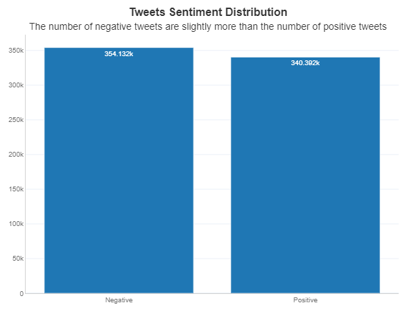
Let's check the distribution of the sentiment labels in the dataset.
Text Preprocessing
First, we will create a set of stopwords which contain common words that we want to remove from the tweets. Removing stopwords can reduce the size of the dataset and also minimize the noise in the dataset, however we should choose the stopwords carefully for sentiment analysis. For example, the word "not" is often regarded as a stopword, but it is actually important for sentiment analysis. We do not want the sentences "I am not happy" and "I am happy" to be treated as the same by our model. You can view the custom stopwords that we use here. We also create an instance of WordNetLemmatizer from the NLTK library, which will be used to convert words into their base form while considering the context.
The text prepocessing consists of the following steps:
- Converting the text to lowercase
- Expanding negative contractions (n't to not)
- Removing URLs
- Removing usernames
- Removing HTML entities
- Removing characters that are not letters
- POS tagging the words (to get better lemmatization results)
- Excluding words with only 1 character and stopwords
- Lemmamatizing the remaining words
Some examples of the preprocessed tweets are shown below.
| tweet | cleaned_tweet |
|---|---|
| I am not very happy with the quality of the coffee from @ExampleShop, wouldn't be buying it anymore | not very happy quality coffee not buy anymore |
| www.examplestore.com is running a discount promotion, so I bought several t-shirts there. Quite satisfied with the quality of the products. | run discount promotion buy several shirt quite satisfied quality product |
Splitting and Tokenization
Before splitting the dataset, we will drop any rows where the cleaned_tweet column is empty. Then, we will divide the dataset into training set (80%) and test set (20%). We will use the training set to train the model, and the test set to evaluate the performance of the final model.
The distribution of the sentiment labels in the training set and test set are relatively similar.
Training set sentiment distribution
Negative: 283011 (50.9%)
Positive: 272608 (49.1%)
Test set sentiment distribution
Negative: 71121 (51.2%)
Positive: 67784 (48.8%)
We then extract the feature (X) and target (y) from the training set. The prior training set is further split into training set (80%) and validation set (20%). The training set will be fitted to the model. The validation set will be used to evaluate the model's performance during training and to make decisions about the training process, e.g. when to stop training (to avoid overfitting) and which model to choose as the final model.
Next we will create an instance of Tokenizer from the Keras library, which will be used to convert the text into a sequence of integers. The tokenizer is fitted to X_train to identify the unique words in the training set and map them to the corresponding integers.
Number of Unique Words: 111001
Machine learning models do not understand text, so we need to convert both X and y into numerical form. We use the fitted tokenizer to convert X_train and X_val into sequences of integers. The sequences are then padded so every sequences have the same length. Notice that we use X_train.shape[1] as the maximum length for X_val to ensure that the length of sequences in X_train and X_val are the same (required by the model). We then perform one-hot encoding on the target labels (y_train and y_val).
Word Embedding and Model Building
We will use a pre-trained GloVe word embedding to create the embedding matrix, which will serve as the weights for the embedding layer. The embedding layer will convert the sequences of integers into sequences of vectors, which will be used as the input to the LSTM layer. To ensure that the pre-trained weights are not modified during training, we set trainable to False for the embedding layer. We keep the pre-trained weights fixed because the GloVe embedding has already been trained on a large corpus of tweets and we want to utilize that pre-trained knowledge.
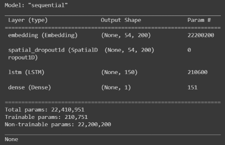
Now we will create our LSTM model. The model consists of the following layers:
- Embedding layer (converts sequences of integers into sequences of vectors)
- SpatialDropout1D layer (prevents overfitting by randomly deactivating neurons)
- LSTM layer (extracts features from the sequences of vectors while considering their order)
- Dense layer with one neuron and sigmoid activation function (outputs the probability of the tweet being positive)
The model is then compiled with the Adam optimizer and binary crossentropy loss function.
Notes: The sentences "I am not happy because today is raining" and "I am happy becuase today is not raining" would be treated the same by a model that does not consider the order of the words (e.g. Naive Bayes algorithm using a unigram bag-of-words model). However, LSTM model can recognize the difference between the two sentences.
Now we are ready to train our model. We set two callbacks to monitor the training process: EarlyStopping and ModelCheckpoint. The EarlyStopping callback will reduce overfitting by stopping the training process if the validation loss does not decrease after 3 epochs. The ModelCheckpoint callback will save the model whenever a new best model is found (based on the validation loss).
After 10 epochs, the model stops training because we only set the epochs to 10. The accuracy and loss of the model on the training set and validation set are shown below. The validation accuracy and loss kind of level off after 7 or 8 epochs.
Notice that the validation accuracy is always higher than the training accuracy, while the validation loss is always lower than the training loss. This is common when using Dropout because regularization mechanism such as Dropout is not applied when evaluating the validation set.

Evaluation on Test Set
We will choose the model with the lowest validation loss as the final model (model on epoch 8), then evaluate its performance on the test set. Remember that we need to convert the cleaned tweets in the test set into sequences of integers and pad them before feeding them to the model. The output of the model is the probability of the tweet having a positive sentiment, so we will convert the probability into a label by setting the probability threshold to 0.50.
The accuracy on test set (78.6%) is similar to the accuracy of the validation set (79.0%), which means the model can generalize well to unseen data.
0.7855224793923905
The true negative rate is higher than the true positive rate, which means that the model is a bit biased towards predicting negative sentiment.
True Negative Rate: 0.812 True Positive Rate: 0.758
We have performed text preprocessing and build a LSTM model that can predict the sentiment of tweets. In the next post, we will create a Streamlit app that can predict the sentiment of tweets and show some visualizations based on a given search term.
Hope you enjoyed the post!
Further reading
Read More
1. Data Collection | Twitter (X.com) Sentiment Analysis
End-to-end machine learning project on sentiment analysis. In this post, we will walk through the data collection process with distant supervision method.
3. Model Deployment w/ Streamlit | Twitter (X.com) Sentiment Analysis
End-to-end machine learning project on sentiment analysis. In this post, we will walk through the steps of creating a dashboard and deploying our model as a web app with Streamlit.
4. Use Cases | Twitter (X.com) Sentiment Analysis
In this final installment, we will explore some use cases of Twitter sentiment analysis in the field of business and social science.
Tags: lstm, machine-learning, sentiment-analysis, nlp, deep learning