AI for Plant Disease Detection

Intro

The dataset used in this article is derived from aerial imagery of Chinese cabbage fields. It consists of image patches, sizing 150 x 150 pixels each, which are categorized into three distinct classes: background, diseased, and healthy.

To begin with, let's do the usual Python import required for processing the images.

Dependencies and Setup

import os
import torch
import pandas as pd
import numpy as np
import matplotlib.pyplot as plt

from tqdm import tqdm
from sklearn import metrics
from PIL import Image
from torch import nn
from torchvision import transforms

GPU Check

We recommend to use GPU to achieve faster training. However, the codes in this article will work just fine on a CPU. To check whether PyTorch is correctly installed and has access to GPU, you can run the code below:

if torch.cuda.is_available():
    device = torch.device("cuda")
    print(f"CUDA is available. Using GPU: {torch.cuda.get_device_name(0)}")
else:
    device = torch.device("cpu")
    print("CUDA is not available. Using CPU.")

print(f"Selected device: {device}")

CUDA is available. Using GPU: NVIDIA GeForce RTX 3050 Selected device: cuda

If you have a CUDA-compatible GPU, it will be printed as shown above.

Prepare the Dataset

The images are organized into three folders based on their class labels: background, diseased, and healthy. They are my own drone-captured images of a Chinese cabbage field, taken in Korea as part of my academic research. The image collection process begin with an in-field survey, upon which disease symptoms were visually detected and confirmed. All images captured during this survey are done between 11am and 1pm so the lighting conditions are consistent.

This is my current directory structure:

.
├── dataset/
│   ├── background/
│   ├── diseased/
│   └── healthy/
│
└── trainer.ipynb

Store the Image Directories on Memory

Firstly, we need to store the image paths in memory. A convenient way to do this is by using the pandas library to create a DataFrame. This DataFrame will have two columns: image_directory, which will hold the full path to each image file, and class_id, which will represent the category (e.g., background, diseased, healthy) each image belongs to.

# Define these 3 classes
CLASSES = ["background", "diseased", "healthy"]

# Create a function to loop through the dataset directories and store the image directory and its class
def getImages(dataset_dir: str) -> pd.DataFrame:
    images = []

    for class_name in os.listdir(dataset_dir):
        img_dir = os.path.join(dataset_dir, class_name)

        for img in os.listdir(img_dir):
            img_path = img_dir + "\\" + img
            images.append([img_path, CLASSES.index(class_name)])

    return pd.DataFrame(images, columns=["img_path", "class_id"])

# Print out the number of data points for each class
all_img_df = getImages("dataset")
all_img_df['class_id'].value_counts()

class_id
0    4629
2    3348
1     513

The class_id numbers correspond to the following classes:

• 0: background
• 1: healthy
• 2: diseased

Looking at the number of the data points for each class, it seems like we are dealing with the case of an imbalance dataset. A model developed on imbalanced dataset is likely to be biased, producing predictions that favor the class with the most data points.

There are a couple of ways to deal with this problem, such as truncation, upsampling, and data augmentation. While each approach have their pros and cons, let's start off with the most straight forward one, truncation. Here, we cut-off the excess data points from the background and healthy class to only 1500 data points.

Sampling

# Prepare an empty list to store dataframe for each class
all_img_df_sample = []
for i in range(3):
    if i != 1:
        # Limit the number of data points for background and healthy classes
        df_sample = all_img_df[all_img_df['class_id'] == i].sample(1500)
    else:
	    # Keep the number of diseased samples as it is
        df_sample = all_img_df[all_img_df['class_id'] == i]

	# Append to the storage list
    all_img_df_sample.append(df_sample)

# Concatenate the sampled dataFrames
all_img_df_sample = pd.concat(all_img_df_sample)
all_img_df_sample['class_id'].value_counts()

class_id
0    1500
2    1500
1     513

While this dataset is not perfectly balanced, this distribution accurately reflects the reality within the domain of Plant Pests and Diseases. In practice, the number of healthy samples are often always greater than the number of the diseased ones. Diseased samples typically constitute only 10-30% of the total population, which in practice makes the process of gathering diseased samples in itself a challenge.

Split to Train and Test Set

Divide it into train and test set with a 7:3 ratio.

train_img_df = all_img_df_sample.sample(frac=0.7, replace=False, random_state=1)
test_img_df = all_img_df_sample.drop(train_img_df.index)

train_img_df['class_id'].value_counts(), test_img_df['class_id'].value_counts()

(class_id
0    1049
2    1045
1     365
Name: count, dtype: int64,
class_id
2    455
0    451
1    148
Name: count, dtype: int64)

Using PyTorch's Dataset & DataLoaders

With our DataFrame of image directories ready, the next step is to load and process the images for model training. In PyTorch, this is efficiently handled using the Dataset[1] and DataLoader[2] classes.

We will create a custom dataset by defining a new class that inherits from torch.utils.data.Dataset. This custom class will contain all the logic necessary to open the images and perform any required operations before they are fed into the model.

class Img(torch.utils.data.Dataset):
    def __init__(self, img_df):
        self.img_df = img_df

    def __len__(self):
        return len(self.img_df)

    def __getitem__(self, idx): # Pass the index argument
        # Get the image path on the designated index
        img_path = self.img_df['img_path'].iloc[idx]

        # Open the image using PIL. This is recommended in pytorch documentation since the following transform
        # function process image with PIL type
        image = Image.open(img_path)

        # Define transform function
        preprocess = transforms.Compose([
            transforms.Resize(299),
            transforms.CenterCrop(299),
            transforms.ToTensor(),
        ])

        # Use the defined transform function to transform the image
        image_tesor = preprocess(image)

        # Get the image label
        label = self.img_df['class_id'].iloc[idx]

        # Return both image_tensor (x) input, and label (y) target
        return image_tesor, label

The core functionality lies in the __getitem__ method. Each time the dataset is accessed, the operations defined in this method are executed. This makes it a highly flexible way to manipulate our dataset, allowing us to perform nearly any kind of transformation or processing.

With our custom dataset class prepared, we can now create training and testing dataset instances and load them using DataLoader.

# Instantiate both training and testing Dataset
train_ds = Img(img_df=train_img_df)
test_ds = Img(img_df=test_img_df)

# Set the batch size to 32. Optionally, you can increase it for faster training
BATCH_SIZE = 32

# Load the train and test Dataset to pyTorch DataLoader
train_loader = torch.utils.data.DataLoader(dataset=train_ds, batch_size=BATCH_SIZE, shuffle=True)
test_loader = torch.utils.data.DataLoader(dataset=test_ds, batch_size=BATCH_SIZE, shuffle=True)

Prepare the Model

For simplicity purposes, we're going to pick a ready-to-use architecture inception_v3 as our plant disease detection model. Using pretrained inception_v3 model means that this model has already been trained using ImageNet dataset and have its weights 'learned' useful image features.

However, to actually makes it applicable for our use case, the model needs to be tuned to 'adapt' to our dataset. This approach is commonly known as transfer learning approach.

To execute this approach, the last fully-connected (FC) layer has to be 'cut-out' and replaced with a new FC layer. This new FC layer is supposed to have the 3 outputs (nodes) in this case, for background, diseased and healthy class.

For the training, we will:

• Use CrossEntropyLoss as the loss function.
• Optimize with Stochastic Gradient Descent (SGD).

While most modern approaches rely on the Adam optimizer, starting with SGD is a solid choice to understand the fundamentals of optimization.

LEARNING_RATE = 1e-04

# Load architecture and pretrained weights of inception_v3 model
model = torch.hub.load('pytorch/vision:v0.10.0', 'inception_v3', pretrained=True)

# 'Cut-off' the top of the model, the last fully connected layer and attach the new one, a FC with only 3 nodes
model.aux_logits = False
num_features = model.fc.in_features
model.fc = nn.Linear(num_features, 3)
model = model.to(device) # Make sure that it will do the computation on GPU

# Define loss function
criterion = nn.CrossEntropyLoss()

# Use SGD optimizer
optimizer = torch.optim.SGD(model.parameters(), lr=LEARNING_RATE, momentum=0.9)

Prepare Utility Functions

Before diving into the core task, let's create a few utility functions to help us in performing a last minute dataset inspection and later on to evaluate our model's prediction.

Prediction Function

This function puts the model in evaluation mode, disables gradient calculations, and for each batch of data, it performs a forward pass to get predictions. Then, the true and predicted labels are gathered and returned as two separate NumPy arrays.

def predictDataset(loader: torch.utils.data.DataLoader, model: torch.nn.Module) -> Tuple[np.ndarray, np.ndarray]:
    actual = np.array([])
    prediction = np.array([])
    model.eval()

    with torch.no_grad():
        for x, y in loader:
            x = x.to(device=device)
            y = y.to(device=device)

            scores = model(x)
            _, predictions = scores.max(1)
            actual = np.append(actual, y.cpu().detach().numpy())
            prediction = np.append(prediction, predictions.cpu().detach().numpy())

    return actual, prediction

actual, prediction = predictDataset(test_loader, model)

(array([0., 0., 0., ..., 2., 2., 2.], shape=(1054,)),
    array([0., 0., 2., ..., 2., 2., 2.], shape=(1054,)))

Confusion Matrix

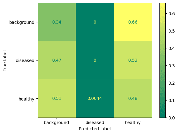
This function plots the prediction into a confusion matrix, which is a simple yet effective way of showing prediction performance of each class. When you create a confusion matrix prior to the training phase, it serves as a baseline to compare against after the model has been trained.

def drawConfusionMatrix(actual, prediction, normalize=True):
    confusion_matrix = metrics.confusion_matrix(actual, prediction)
    cmn = confusion_matrix.astype('float') / confusion_matrix.sum(axis=1)[:, np.newaxis]

    if normalize:
        confusion_matrix = cmn

    cm_display = metrics.ConfusionMatrixDisplay(confusion_matrix = confusion_matrix, display_labels=CLASSES)
    cm_display.plot(cmap='summer')
    plt.show()

drawConfusionMatrix(actual, prediction)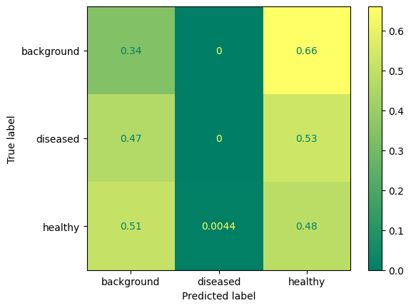

Display images

We shall also create a helper function to display sample images. It does a quick last-minute check to ensure that the dataset preprocessing and model creation are functioning correctly.

def displayImgs(imgs, predicted_labels, true_labels, classes, n):
    max_img_num = 12
    n = n if n <= max_img_num else max_img_num
    ncols = 4
    nrows = n // ncols

    fig = plt.figure(figsize=(16, 9))  # Adjusted figure size
    for i, tensor in enumerate(imgs[:n]):
        img = tensor.permute(1, 2, 0).cpu().numpy()

        title = (
            f"True class     : {classes[true_labels[i]]}\n"
            f"Predicted class: {classes[predicted_labels[i]]}"
        )

        ax = fig.add_subplot(nrows, ncols, i + 1)
        ax.imshow(img)
        ax.set_title(title, fontsize=10, fontfamily="monospace", loc='left')
        ax.axis('off')

    plt.subplots_adjust(hspace=0.6)
    plt.show()

model.eval()  # Evaluation mode
with torch.no_grad():
    x, y = next(iter(train_loader))
    x, y = x.to(device), y.to(device)

    logits = model(x)
    model_pred = logits.argmax(dim=1)

    displayImgs(x, model_pred, y, classes=CLASSES, n=BATCH_SIZE)

Evaluation Function

Loop through the dataset loader and feed each batch to the model. It gives us model's prediction, which then calculates the number of correct predictions (overall accuracy).

def evaluate(loader, model, criterion):
    model.eval() # Evaluation mode

    # Prepare list to store predictions and set initial val_loss
    actuals, predictions = [], []
    val_loss = 0

    with torch.no_grad():
        for x, y in loader:
            x, y = x.to(device), y.to(device)

            scores = model(x)
            preds = scores.argmax(dim=1)

            actuals.append(y)
            predictions.append(preds)

            loss = criterion(scores, y)
            val_loss += loss.item()

    actuals = torch.cat(actuals)
    predictions = torch.cat(predictions)

    # Calculate overall accuracy
    oa = (actuals == predictions).float().mean().item()

    # Calculate overall loss
    ol = val_loss / len(loader)

    return oa, ol

Training

This section is the (almost) final step of the pipeline, all the preparation up to this point—building image patches, validating the dataset, and loading the model—is to embrace the black box. We are now quite sure that we prepared the dataset (image patches) as intended, loaded the model and they all worked correctly.

The objective of this step is to fine-tune the pretrained inception_v3 model weights.

In PyTorch, the training process is typically more explicit than in TensorFlow. It involves iterating over the dataset, performing forward passes to generate predictions, resetting gradients, updating the model's weights, and repeating these steps for each batch and epoch.

NUM_EPOCHS = 50

# Prepare list to store loss and accuracy data
train_losses = []
test_losses = []
train_accuracy = []
test_accuracy = []

for epoch in range(NUM_EPOCHS):
    model.train()  # Training mode
    batch_losses = []
    correct = 0
    total = 0

	# Use tqdm for a cool progress bar
    loop = tqdm(enumerate(train_loader), total=len(train_loader))
    for batch_idx, (data, targets) in loop:
        data, targets = data.to(device), targets.to(device)

        # Forward pass
        scores = model(data)
        loss = criterion(scores, targets)

        # Backward + optimize
        optimizer.zero_grad()
        loss.backward()
        optimizer.step()

        # Track training loss
        batch_losses.append(loss.item())

        # Compute train accuracy for this batch
        preds = scores.argmax(dim=1)
        correct += (preds == targets).sum().item()
        total += targets.size(0)

        # Update progress bar
        loop.set_description(f"Epoch[{epoch}/{NUM_EPOCHS-1}]")

    # Calculate current's epoch stats
    epoch_train_loss = np.mean(batch_losses)
    epoch_train_acc = correct / total
    train_losses.append(epoch_train_loss)
    train_accuracy.append(epoch_train_acc)

    # Evaluate on test set
    epoch_test_acc, epoch_test_loss = evaluate(test_loader, model, criterion)
    test_accuracy.append(epoch_test_acc)

    print(f"Train Loss={epoch_train_loss:.4f}, Train Acc={epoch_train_acc:.4f}, "
          f"Test Loss={epoch_test_loss:.4f}, Test Acc={epoch_test_acc:.4f} \n")

    Epoch[0/49]: 100%|██████████| 77/77 [00:36<00:00,  2.11it/s]
	Train Loss=0.8599, Train Acc=0.7015, Test Loss=0.7698, Test Acc=0.7979

	Epoch[1/49]: 100%|██████████| 77/77 [00:35<00:00,  2.17it/s]
	Train Loss=0.7205, Train Acc=0.7780, Test Loss=0.6499, Test Acc=0.8083

	Epoch[2/49]: 100%|██████████| 77/77 [00:35<00:00,  2.16it/s]
	Train Loss=0.6080, Train Acc=0.7983, Test Loss=0.5631, Test Acc=0.8150
	...

	Epoch[47/49]: 100%|██████████| 77/77 [00:33<00:00,  2.29it/s]
	Train Loss=0.0227, Train Acc=0.9967, Test Loss=0.5225, Test Acc=0.8539

	Epoch[48/49]: 100%|██████████| 77/77 [00:33<00:00,  2.31it/s]
	Train Loss=0.0277, Train Acc=0.9951, Test Loss=0.5153, Test Acc=0.8520

	Epoch[49/49]: 100%|██████████| 77/77 [00:33<00:00,  2.30it/s]
	Train Loss=0.0162, Train Acc=0.9988, Test Loss=0.5183, Test Acc=0.8520

The final testing accuracy is 0.8520, which is a solid result for an initial model.

An experienced deep learning practitioner might point out that the training setup—such as the learning_rate, batch_size, epochs, and similar parameters—could be optimized further. More advanced techniques such as early stopping and checkpoints could also be beneficial.

Accuracy & Loss Plots

epochs = range(NUM_EPOCHS)

plt.figure(figsize=(12,5))

# Accuracy plot
plt.subplot(1,2,1)
plt.plot(epochs, train_accuracy, label='Train Accuracy')
plt.plot(epochs, test_accuracy, label='Test Accuracy')
plt.ylim(0, 1.05)
plt.xlabel('Epoch')
plt.ylabel('Accuracy')
plt.title('Train vs Test Accuracy')
plt.legend()
plt.grid(True)

# Loss plot
plt.subplot(1,2,2)
plt.plot(epochs, train_losses, label='Train Loss')
plt.plot(epochs, test_losses, label='Test Loss')
plt.xlabel('Epoch')
plt.ylabel('Loss')
plt.title('Train vs Test Loss')
plt.legend()
plt.grid(True)

plt.show()

Because we are using the weights of the final model, the above accuracy and loss plot suggest that the model may have slightly overfitted. While the training logic could certainly be improved, we shall keep this article concise and won't dive into those adjustments here.

There are a couple of good articles demonstrating better training strategies [3], [4] [5].

The Confusion Matrix

With the training done, let us now evaluate the model's performance using the confusion matrix. This will help us understand how well the model is performing across different classes.

actual, prediction = predictDataset(test_loader, model)
drawConfusionMatrix(actual, prediction, normalize=True)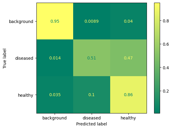

Key analysis:

• The background class having more distinguishable features compared to the other two, achieved 95% correct prediction, is the easiest to recognize.

• The healthy class is predicted correctly 86% of the time, although 10% are incorrectly classified as diseased.

• The diseased class however is only correctly predicted 51% of the time in test samples; nearly half (47%) are misclassified as healthy. This indicates that the model may not be sensitive enough to detect diseased leaf.

Display Predictions

Iterate over the train_loader once, then display it using displayImgs function to visualize the model's predictions.

model.eval()
with torch.no_grad():
    x, y = next(iter(train_loader))
    x, y = x.to(device), y.to(device)

    logits = model(x)
    model_pred = logits.argmax(dim=1)

    displayImgs(x, model_pred, y, classes=CLASSES, n=BATCH_SIZE)

Save the Model

In PyTorch, you can save the weights with torch.save(), and load them later with torch.load(). When loading the weights, you need to ensure that the model architecture is defined in the same way as it was during training.

torch.save(model.state_dict(), "inception_v3_plant_disease.pth")

Application

Imagine that we are working a large aerial orthomosaic image of a farm field -- potentially several gigabytes in size -- it is rich in information but memory-expensive to process it in blob. To handle this, we need to process it in manageable size of chunks, for example, 2000 x 2000 pixels each.

Assuming we already have the necessary patches extracted, we shall demonstrate how to process these patches for inference, before aggregating these predictions to visualize a heatmap where diseased areas are highlighted.

import segmentor as sg

# Initialize segments
segments = sg.initSegments(chunk_id=14)

# Define transform function, exactly the same with the one we used in Img class
transform = transforms.Compose([
    transforms.Resize(299),
    transforms.CenterCrop(299),
    transforms.ToTensor(),
])

# Loop through segment_ids
for segment_id in range(1, segments.segments.max()):

	# This function further 'cut' the image chunk into patches with max size of 150 x 150 pixels
    patch = segments._patchBuilder(segment_id)

    if patch is not None:
	    # Convert to pill image then transform
        PIL_patch = Image.fromarray(patch[..., ::-1]) # Reverse the channel order
        input_tensor = transform(PIL_patch)

		# The model expect 4D tensor with Shape: (batch, channel, height, width)
        input_tensor = input_tensor.unsqueeze(0)

		# Make sure the model in evaluation mode
		model.eval()
        with torch.no_grad():

			# Feed the patch tensor
            output = model(input_tensor.to(device=device))
            pred_class = output.argmax(dim=1).item()

			# Colorize the patch according to the predicted class
			# Background: Purple
			# Diseased: Red
			# Healhy: Green
            segments.colorize(pred_class)

plt.imshow(segments.image[..., ::-1])

plt.imshow(segments.image_classified[..., ::-1])

Takeaways

We have successfully developed a working inception_v3 model with 0.85 overall accuracy to correctly classify background, diseased and healhy of Chinese cabbage field images. However, it may need some improvements to make it more sensitive for detecting diseased leaves, as it was only able to correctly classify 51% of the diseased samples.

Nevertheless, we can use this initial experimentation as a foundation for further development and refinement. This might involve collecting more diverse training data, fine-tuning the model architecture, dataset augmentation, and experimenting with different hyperparameters to improve performance. In present day research, more advanced techniques that leverage transfer learning, self-supervised learning, and ensemble methods are being explored to enhance model robustness and accuracy.

Since large orthomosaic images cannot be processed all at once, the final application we develop must also incorporate a strategy of patch-based processing. This solution requires a method to divide them into smaller, analyzable patches. Our model could then process each patch independently, even defining the stages of infection (e.g. mild, medium, severe) for each patch in the context of the overall image.

The repertoire of techniques available for patch-based processing is vast, including methods for efficient data loading, augmentation strategies tailored to small image regions, and specialized neural network architectures designed to handle variable input sizes. When working with a consultant like Supertype, it is often the case of leveraging the existing body of knowledge and tools in the ecosystem to aid in the development of a plant disease detection system that is time-efficient and scalable.

Keep reading

Data Science in Industry

Data Science in Industry

Unlocking Efficiency: The Importance of Predictive Maintenance

Explore how predictive maintenance powered by AI is transforming industries like mining and manufacturing by reducing costs and minimizing downtime.

LWVC

Lukas Wiku, Vincentius C. Calvin

14 min read

Data Science in Industry

Data Science in Industry

AI for Rail Transportation

A high level guide on how AI is used in rail transportation industry meant for executives and decision makers.

SC

Samuel Chan

13 min read

Data Science in Industry

Data Science in Industry

Data Science for Digital Advertising

How I use data analytics to deliver value to my advertising clients; A case study on creative decay analysis, retention rate analysis, and exploratory data analysis (python code provided)

GB

Gerald Bryan

8 min read

Field notes, straight to your inbox

We publish what we learn building analytics and AI systems for some of the largest enterprises in the region. Subscribe and we will send the next one your way.

The latest in AI and Enterprise Analytics

Email addressSubscribe

We do not resell your data. We respect your privacy and trust.