Data Warehouse Modernization w/ BigQuery
A detailed documentation on building a modern data warehouse in BigQuery featuring storage and performance optimization.
Feb 25, 2025 · Stane Aurelius
In a typical data processing architecture, data warehouse is probably the most commonly used service, making it one of the most important things to be familiar with for every data practitioner. After all, data warehouse is the starting point of data consumption — it consolidates raw data coming from various sources and shares them across all of the applications that are usually used to generate reports, dashboards, etc. However, the process of setting up and configuring a data warehouse is no mean task. The capability of being able to store and organize big data is only the tip of the iceberg, while the crux of the matter lies in optimizing the data warehouse for simplicity and access and high-speed query performance. Without effective data sharing capabilities, every application in a data processing architecture that relies on the data contained in a data warehouse will be in dire straits.
Numerous data warehousing solutions are currently available on the market. For this article, we will be discussing about a data warehouse named BigQuery in particular. In a nutshell, this data warehouse provided by Google Cloud has a lots of implemented features which deemed it to fulfill the requirements of a modern data warehouse, which are but not limited to:
- Autoscaling up to petabytes of data
- Serverless and Fully-Managed
- Supports integration with ETL and data processing tools
- Machine Learning in SQL
- Data and queries collaboration
Despite its capabilities, learning BigQuery should only require little (if not none) prior experience, and it is a fine tool to be added to your toolbox. Furthermore, you can always experiment things by creating a Google Cloud Platform account (Google will also give you free trial credits that you can use to try out all of their services).
Introduction to BigQuery
Let's begin by looking at the structure of BigQuery. Just like every other data warehouses, data tables in BigQuery are organized and divided into multiple data marts called datasets. It is helpful to think of them as a collection of shelves in a warehouse, each storing a different collection of items. In a real-world scenario, datasets are often siloed by departments. Thus, as a general rule of thumb, group the data tables based on the domain the data pertains to for the purposes of:
- Structuring information logically
- Isolating datasets from each other according to business needs
- Saving the time it needs to search and retrieve a particular data
Creating a dataset in BigQuery is quite straightforward. Under SQL Workspace, click on the three dots menu on the right side of your project name and select Create Dataset. Provide any name of your choice for the dataset ID.
In a real-world scenario, you would want to choose a location that is either closest to you (for lower latency), or one that complies with your business requirements. However, as we will be using a provided BigQuery dataset for a demonstration, choose
US multi-regionas the dataset location instead. I will explain why we need to do this in the later section of this article.
Upon creating a dataset, you can directly create some data tables in BigQuery and play around with them to better familiarize yourself. "But hey, I do not have any data available! Where can I get some data that is recommended for practice?" is one of the major problems people encounter when learning a new database system. Fortunately, Google Cloud has provided some public data which you can directly access in BigQuery! Try to click on the + ADD DATA button on the right side of Explorer and click on the Public Datasets option. Lots of options would come up in the marketplace! As of now, search for NYC City Bike Trips and click on View Dataset.
You should see the NYC Citi Bike Trips dataset info on your screen. What you need to do is copy the dataset ID and paste it into the search bar under Explorer. If the explorer shows no result, click on Broaden search to all and you should see the new_york_citibike dataset containing 2 tables: citibike_stations and citibike_trips. Try to click on the citibike_trips table! See that BigQuery provides the schema, details, and preview of the data table.
you can star the
bigquery-public-dataproject so that it is always shown in the explorer panel. Once it is shown in the explorer panel, you can also see all of the datasets and tables contained within.
While the citibike_trips is (in my opinion) one of the perfect data for learning, the size of the data is too big. Take a look at the table details and you should notice that it contains 7.47 GB data with around 58 million rows! When you are using BigQuery, the first 1 TB of query data processed is free per month. But you do not want to waste this free quota just for practice right? So as to not incur unnecessary costs, we will do a quick sampling and copy 15% of the citibike_trips table into our previously created dataset. Change the <project_name> and <dataset_name> and run the following query in your BigQuery editor!
Copying tables is only possible between 2 datasets with the same region. Most BigQuery public dataset are stored in US multi-region, hence the reason why we set our dataset's region. If you insist on copying tables cross-region, you might want to explore more about BigQuery transfer service.
At this point, your dataset should contain a table named bike_trips with almost 8 million rows. Notice that everytime you write a query, BigQuery will tell you how many bytes it will process to execute it on the top right side of the editor panel. Under the hood, analytics throughput is measured in BigQuery slots. It would be easier to comprehend BigQuery slots by regarding them as a combination of CPU, memory, networking resources, and a number of supporting sub-services for executing SQL queries. Everytime you write a query, BigQuery automatically calculates how many slots are required at each query stage depending on the size and complexity. Let's try to perform an aggregation: suppose we are trying to solve "on average, how many minutes do subscribers' bike trips last in every month of every year?"
Fun fact: when writing queries in BigQuery, you can actually split the editor and schema tab. This way, you can just click on the column name on the schema tab when you want to reference it in your query!
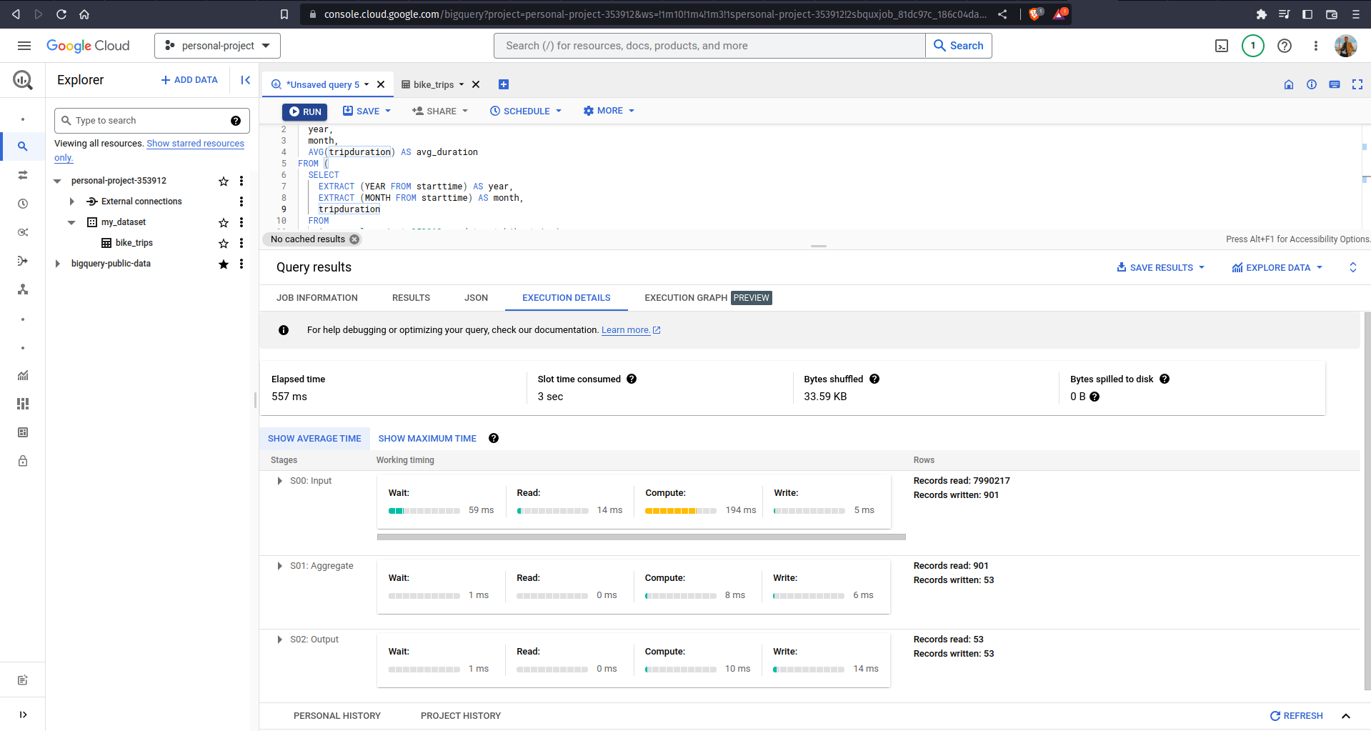
If you click on the EXECUTION DETAILS tab, you can see the process/stages of going from almost 8 million records to 53 records output. Another interesting information in this tab would be the Slot time consumed — from the picture above, it means that if a computer did all of the processes linearly, it would take 3 seconds to finish the job; while BigQuery only takes 557 ms (see the Elapsed time) to finish it due to distributed parallel processing. Now you might be thinking "Am I learning all this stuff just to save about 2 seconds in running queries?" Well, we only did a demonstration on a small size of data, so the result might seem insignificant. There was a demo on using BigQuery to perform aggregation on a 700 GB dataset with over 10 billion records. The execution details showed a Slot time consumed of 2.5 hours, and the elapsed time was just about 10 seconds! Talk about the beauty of distributed parallel processing.
BigQuery Connections
Among the various services offered in Google Cloud Platform, BigQuery might be the one with the most number of available connections — you can connect various data sources and processing tools with BigQuery. Let's first talk about different ways to ingest data into BigQuery. Normally, we would already have a data lake that stores our raw data before it is consolidated. The method to load all of this data depends on how much transformation is needed:
-
EL (Extract and Load)
This method is suitable for raw data with the same schema as the destination table and able to be imported as is.
-
ELT (Extract, Load, Transform)
In this method, raw data will be loaded into a destination table and transformed afterwards. This method is suitable for data that requires simple transformations — use standard SQL DML (Data Manipulation Language) to perform transformations on the data.
-
ETL (Extract, Transform, Load)
ETL requires the data to go through an intermediate transformation process before being loaded into the destination table. In Google Cloud Platform, the commonly used intermediary services for data transformation are Dataproc and Dataflow.
Regardless of the necessary transformations, there are multiple ways of ingesting data into BigQuery. For periodically loading batch data, the most straightforward way is by clicking the three dots menu on a dataset, click on Create Table, and choose the corresponding data source. But this method is not so efficient right? Whenever the data is updated, you always need to intervene with the loading process. For the case of automation, there are 2 solutions:
-
Transfer data to Cloud Storage in formats that are supported by BigQuery (CSV, Avro, Parquet, etc) and set up Cloud Functions to listen to a Cloud Storage event associated with new files arriving in a given bucket. This way, Cloud Functions will act as a sensor that triggers a BigQuery load job when new data arrives in a bucket.
-
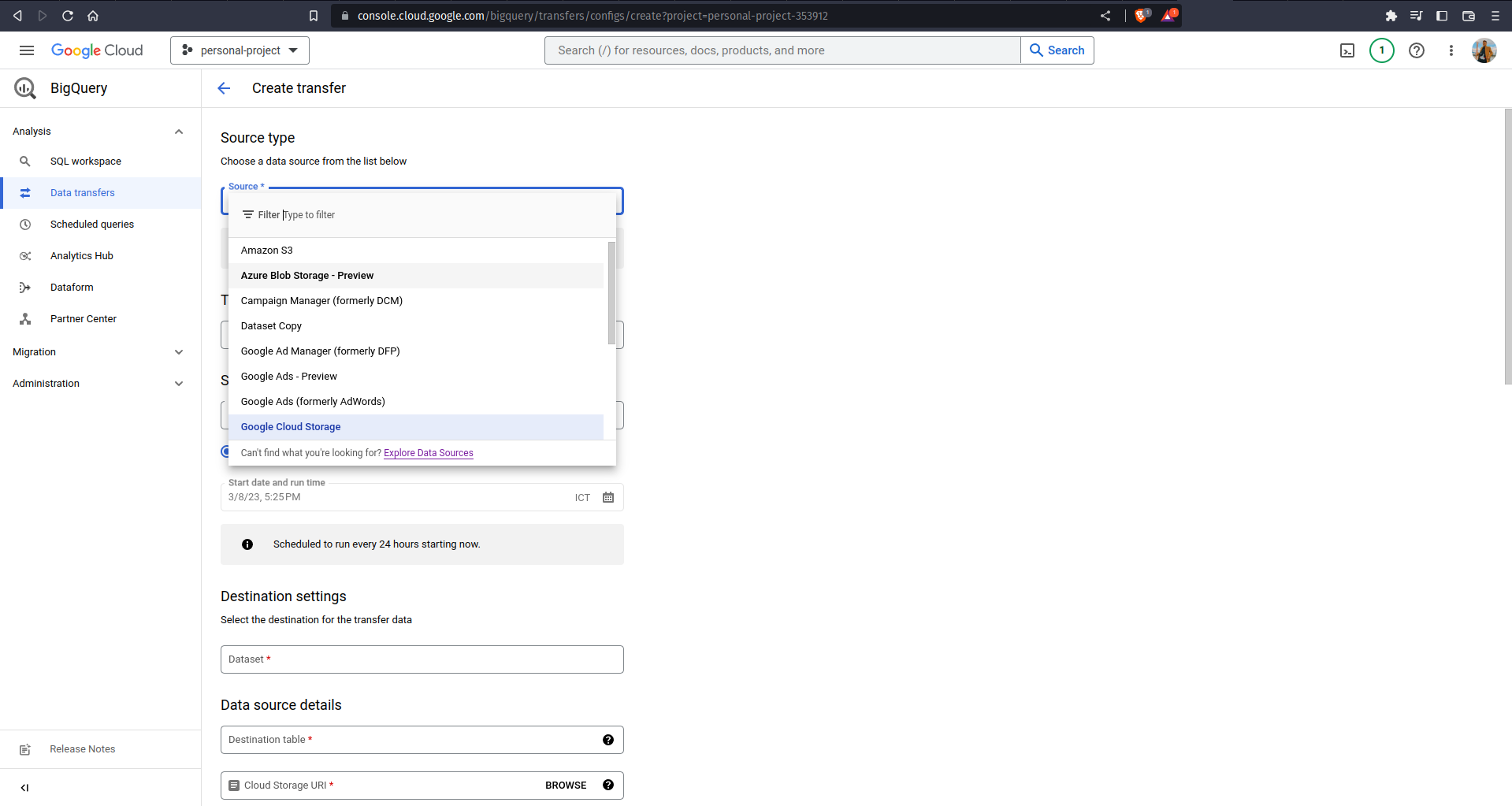
Use BigQuery Data Transfer Service to schedule an automated data transfer from wherever the data is located into BigQuery. Click on the Data Transfers tab to see a list of the available data sources, it even includes Amazon S3, Youtube Channels, Google Play, and many others!
If your raw data is stored in Cloud SQL or Cloud Spanner, you can directly access the data through BigQuery using Federated Queries. Google Cloud provides BigQuery Connection API that can be used to establish a connection to Cloud SQL or Cloud Spanner, and federated queries allow you to send a query statement to external database, receiving temporary tables as a result. To do this, click on + ADD DATA button and click on Connections to external data sources. Specify the connection name and database credentials.
Once you have set up an external data connection, you should be able to see it in the explorer panel. You can now make a federated query with the EXTERNAL_QUERY function such as the following.
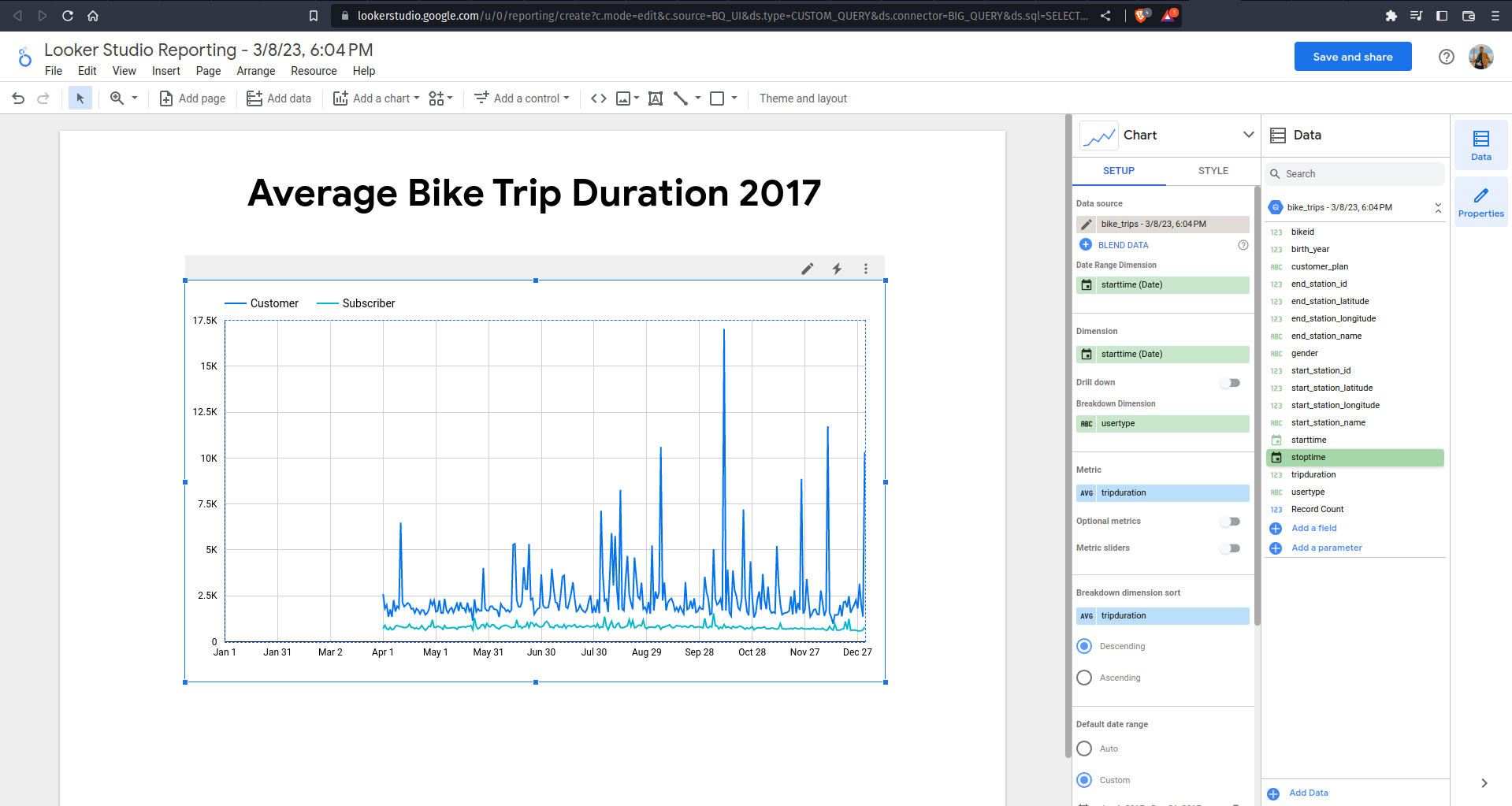
BigQuery also supports connections to other data processing tools! A good example is how you can directly create a report using your query result table. Try to run the following query and click on Explore with Looker Studio on the right side of Query Results
Looker Studio is a tool that you can use to create a report/dashboard. It is very easy to use — just drag and drop any column and you can immediately create nice visualizations! Suppose that we are trying to visualize the average bike trip duration in 2017: we can just specify the tripduration (avg) as metric, usertype as breakdown, specify the custom date range, and voila! Your visualization is all done.
BigQuery can also be connected and used as a data source for other services such as VertexAI, Cloud Composer, etc. However, I will not dive further into those services as the article will get out of topic real quick. For now, as a bit of extra knowledge, the following are the list of aforementioned services and their main usage:
| Service | Usage |
|---|---|
| Cloud Functions | Executing a script based on an event trigger |
| Dataproc | Processing big data with open source software |
| Dataflow | Executing batch and streaming data pipelines |
| Cloud Composer | Orchestrating data workflow |
| Looker Studio | Creating rich visualizations and reporting |
| Vertex AI | Building and deploying Machine Learning models |
These services might get their own articles in the future, so stay tuned to Supertype :wink:
BigQuery Optimizations
While optimizing a data warehouse might be the primary job of a data engineer, getting to understand BigQuery optimizations under your belt will never be a bad thing. Think for a second about what you have learned from the previous section of the article, and I bet you are thinking it is not rocket science — it feels like using a regular database system equipped with a fancy Graphical User Interface (GUI). The true capability of BigQuery goes beyond that! The optimized version is harder to master, and it might be of different shape than a regular database; yet it offers a blazing speed query performance.
Designing Data Warehouse Schema
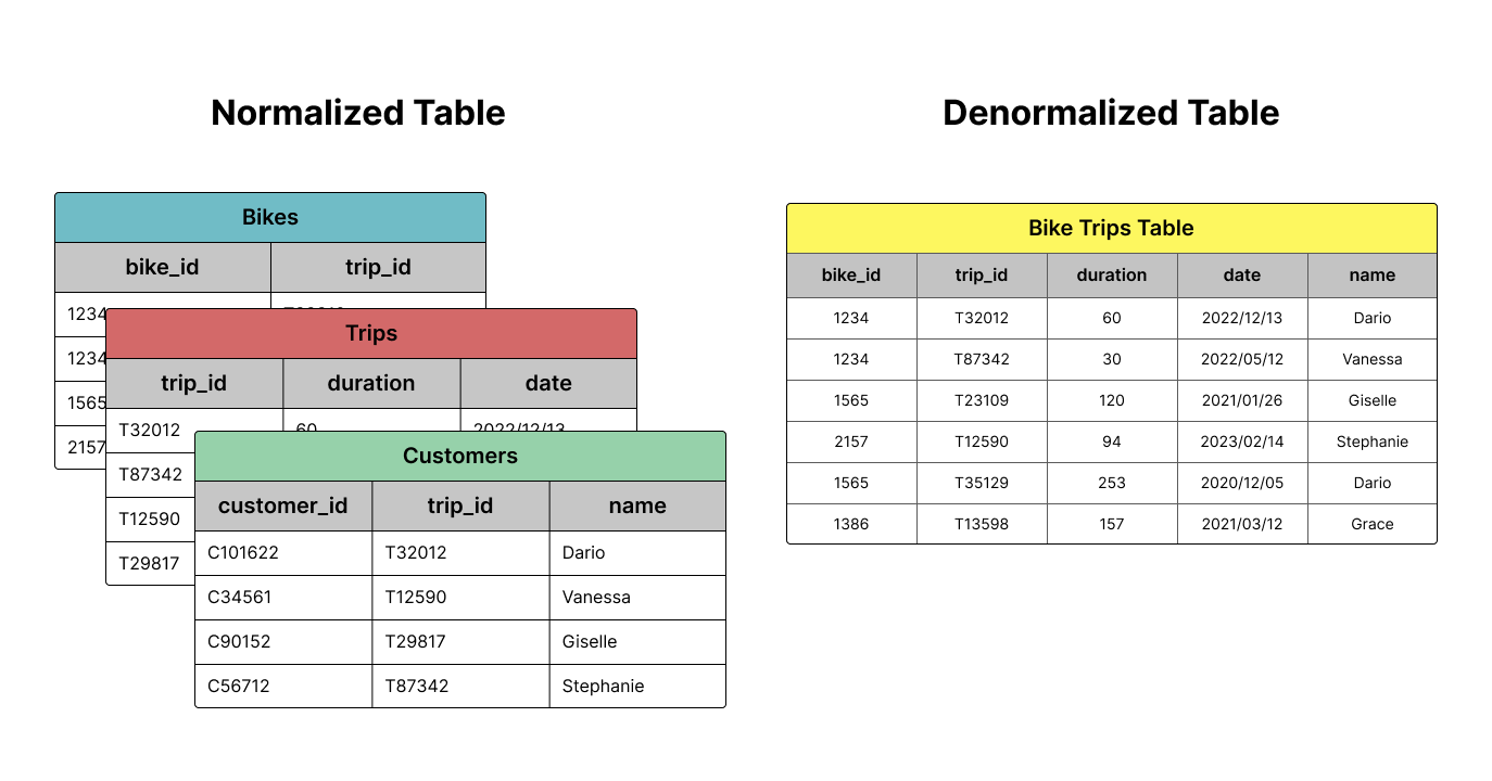
If you have prior experience in managing databases, you might already be familiar with the procedure of normalization. For those who do not, normalizing data means that you are turning it into a relational system — imagine organizing a database into multiple tables. For the case of normalization, several notable impacts for your database are saving up space (removing the number of duplicated records/redundancies) and allowing easier navigation.
On the other hand, denormalization is a contrast strategy that allows duplicate field values for the columns in a table to gain better processing performance. When analyzing normalized data, you would often need to execute JOINS operations, which are being considered expensive due to its requirement of data coordination (hence the necessity of communication bandwidth). On the contrary, flattened data can be processed in parallel using columnar processing because it localizes the data into individual slots. Data warehouses (including BigQuery) are usually columnar since a columnar database is particularly efficient at scanning a column over an entire dataset. That is why you would want to denormalize your data before loading it to BigQuery — remember that sharing data is the main purpose of a data warehouse. Of course, due to the data being repeated instead of being relational, flattened data takes more storage in exchange for query performance. The increase in storage costs is worth the performance gains, not to mention that normalized data has less of an effect in modern database systems.
Nested and Repeated Fields
It is true that denormalizing tables is the recommended practice when using BigQuery, but it is not always rainbows and butterflies either. There are cases where completely flattened data can negatively impact query performance, especially when you need to group the data by a field with one-to-many relationship (bike_id is one such field in our previous data, it has one-to-many relationship with trips). Behind the scenes, BigQuery uses the "shuffle" operation for executing complex aggregation and analytic operations. You can regard the shuffle operation as a data processing pipeline consisting of data repartitioning and transfer over the Google network. The repartitioning part is meant to provide data with minimal fragmentation and overhead that can be read concurrently with high throughput, allowing efficient access and retrieval of relevant rows. Regardless, shuffling is notoriously slow.
For this case of scenario, BigQuery supports columns with nested and repeated fields (commonly referred to as Structs and Arrays, respectively). Array is basically a collection of items with the same data type, while Struct is a key-value pair, similar to a Dictionary in Python. Applying both concepts to the citibike table, the result might look like the following table
| bike_id | year | trips.start_time | trips.end_time |
|---|---|---|---|
| 123 | 2021 | 2021/12/10 08:00:05 | 2021/12/10 10:24:01 |
| 123 | 2022 | 2022/04/02 13:32:40 | 2022/04/02 16:15:05 |
| 2022/07/27 20:45:12 | 2022/07/28 22:10:45 |
Notice that the fields with deeper level of granularity is repeated. The table contains 2 rows. In JSON format, the data will be as shown
The main purpose of structs and arrays is to preserve the relational qualities of the original data and schema while enabling columnar and parallel processing to the fields. Using structs and arrays also enable you to drastically reduce the table size depending on the granularity of the data. Let's try to use it on bigger data bigquery-public-data.chicago_taxi_trips.taxi_trips. Look up the table schema and identify what tables would the data be divided into when being stored in a relational database.
In my opinion, we can divide this data into 4 tables: trip details, payment details, pickup points, and dropoff points. These tables are the ones you need to reconstruct as the arrays of struct.
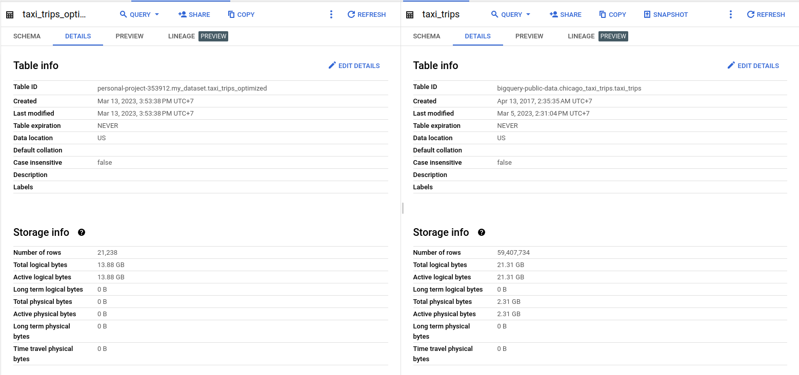
The implementation of structs and arrays results in a 7.43 GB (34.86%) reduction in the data size. Also notice that we are aggregating the data based on company and taxi_id fields, which results in the trip details for each taxi of a company being co-located, hence enhancing the efficiency of the data retrieval.
Partitioning by Field
The last method to optimize BigQuery is by using Partitioning . This method improves the query performance by reducing the number of data read during a query process. You can perform partitioning based on a timestamp, date or datetime field, or a range of integer field (such as ID field). For example, partitioning the bike trips table based on trip_date field obtained by extracting date from starttime field
In the resulting table partitioned by the trip_date column, bigquery will create multiple partitions each containing a single day of data. Because each partition is held in a single physical block, BigQuery needs to maintain more metadata about the properties across all operations that modify it: query jobs, DML (Data Manipulation Language) and DDL (Data Definition Language) statements, load jobs, copy jobs, etc; all for the purpose of accurately estimating the query cost before you run it.
"So how does partitioning increase query performance?" When your query requires filtering values of the partitioning field, BigQuery can directly scan only the partitions that match the filter and skip the remaining partitions. Suppose that you are trying to run a query with a WHERE clause looking for trips that occur between 2017/01/01 and 2017/06/30. Originally, BigQuery will need to scan the entire table and pick those that match the filter. In the partitioned table, however, BigQuery can just directly scan the necessary partitions; so it only needs to scan approximately 180 (total number of days in the where clause) / 1790 (data from 1 July 2013 to 31 May 2018) ≈ 10% of the full dataset, leading to a dramatic cost and time savings. Try to run these 2 queries and compare the execution details.
The first query requires BigQuery to process 2.91 GB of data, while the second query only requires BigQuery to process 256.29 MB of data.

Read More
Introduction to NoSQL
A general introduction to NoSQL databases and their use cases.
Optimizing queries in Postgres and BigQuery
A whirlwind tour of query optimization strategies ft. query plans, index scans, and BigQuery-specific optimizations (part 1 of 2)
Optimizing full text search in Postgres and BigQuery
A discussion on full text search and indexing strategies in Postgres and BigQuery (part 2 of 2)
Querying JSON data in Postgres
Combining the flexibility of JSON with the robustness of a relational database in Postgres.
Tags: Database, BigQuery, Data Engineering