Optimizing queries in Postgres and BigQuery
Read query plans in Postgres and BigQuery, then make queries faster with indexes, partitioning, clustering and fewer scanned columns.
Key Points (TL;DR)
-
Don't optimize a query until you've seen its query plan. In Postgres, that's
EXPLAIN ANALYZE. -
Your most common Postgres queries should run as index scans. On our 1.84 million row test table, an index took a single-row lookup from 13.9 seconds to 0.5 milliseconds ⚡
-
BigQuery has no
EXPLAINand no B-tree indexes. It stores data by column, so what a query costs and how fast it runs depends on how many columns and partitions it reads. -
BigQuery's execution graph and query performance insights show you which stage is slow and why.
-
Select only the columns you need, partition and cluster tables on the columns you filter by, and add a search index for lookups by value.
-
The checklist near the end covers the rest, and the comparison table maps each Postgres tool to its BigQuery counterpart.
The article contains screenshots, benchmark tests, and code snippets for each of these points, so dive right in.
Building optimized analytics applications: from Postgres to BigQuery
This is the first in a series of articles on building highly optimized analytics applications. We're going to start with the basic mental model: thinking about the stack of software that makes up a modern analytics application. We'll see where bottlenecks can occur at each layer of the analytics stack, and work through some concrete examples of how to diagnose and fix them.
Background: The analytics stack
For the purpose of this article, we'll define the analytics stack as the application layers responsible for ingesting, storing and querying data, plus the interface the front end uses for search. Suppose the end users are business analysts who rely on our web application to query for results after they have provided a set of filters and search terms.
This stack is made up of the following components:
- A database for storing the data
- A query engine for querying the data
- A web application for querying the data
A few months into the project, our data analysts start complaining that the web application feels sluggish. Usage of the application has increased, and the analysts are now spending more time waiting for the results of their queries. Where do we start?
Welps! A few discussions with the data architects and analytics engineers on the team reveal that the database might be the bottleneck. In fact, we were told, the team is in the middle of a multi-month migration from an on-premise PostgreSQL database to Google's BigQuery. The migration is still in progress, and we are asked to help diagnose the performance issues in the meantime.
- PostgreSQL: the world's most advanced open source database and perhaps the most popular choice for mature startups
- BigQuery: Google's fully managed and highly scalable data warehouse
In the next few articles of this series, we'll look at each component of the analytics stack in turn, and see how we can diagnose and fix performance issues. Our goal is to build a mental model of the analytics stack, and an overview of the tools at our disposal at each layer. We'll start with the database (first the on-premise Postgres, then BigQuery), and work our way up to the web application layer.
Migrating our database: PostgreSQL to BigQuery
At the bottom of our analytics stack is the database. Currently it is the trusty PostgreSQL database responsible for storing the data and providing an interface for querying it. Being the most fundamental component of the analytics stack, it is naturally the first place to look when diagnosing performance issues.
Fortunately for us, databases today are extremely well optimized for a wide variety of workloads. For the most part, troubleshooting performance in a database means using the tools it already provides:
- the query planner, which decides how to run a query
- the query optimizer, which picks the cheapest of the candidate plans (Postgres bundles it with the planner)
- the execution engine, which runs the chosen plan and can report how long each step took
Let's start off by looking at the query planner of our PostgreSQL database. The query planner takes a query and formulates a plan for how to execute it. PostgreSQL has this to say about the query planner:
The task of the planner/optimizer is to create an optimal execution plan. A given SQL query (and hence, a query tree) can be actually executed in a wide variety of different ways, each of which will produce the same set of results. If it is computationally feasible, the query optimizer will examine each of these possible execution plans, ultimately selecting the execution plan that is expected to run the fastest.
Since the query planner decides how efficiently our queries run, databases let us inspect the plan it chose. This is done with the EXPLAIN command. For example, let's say we have a table called users with the following schema:
CREATE TABLE users (
  id SERIAL PRIMARY KEY,
  name TEXT,
  email TEXT,
  age INTEGER
);
And we have the following query:
SELECT * FROM users WHERE age > 30;We can use the EXPLAIN command to see the query plan for this query:
EXPLAIN SELECT * FROM users WHERE age > 30;Which will output the following:
QUERY PLAN
Seq Scan on users  (cost=0.00..10.00 rows=1000 width=16)
  Filter: (age > 30)
The query plan is a tree structure, where each node represents a step in the execution of the query. In this case, the query plan consists of a single node: a sequential scan of the users table. A sequential scan is the most basic way to read a table. The database reads it from beginning to end and returns the rows that match. The planner falls back to it when it has no better way to execute the query.
The query plan you see will depend on the database you are using and the query you are executing. For example, if you have an index on the age column, the plan will look like this:
QUERY PLAN
Index Scan using users_age_idx on users  (cost=0.00..10.00 rows=1000 width=16)
  Index Cond: (age > 30)
(2 rows)
The plan has changed from a sequential scan to an index scan. An index scan lets the database jump straight to the matching rows instead of reading the entire table, which is why we create indexes for the columns we filter on most.
EXPLAIN shows the plan without running the query. To run the query and see what actually happened, use EXPLAIN ANALYZE:
EXPLAIN ANALYZE SELECT * FROM receipts WHERE amount > 5000;Which will output the following (again, assuming we have an index on the amount column):
QUERY PLAN
Index Scan using receipts_amount_idx on receipts  (cost=0.00..10.00 rows=1000 width=16) (actual time=0.012..0.012 rows=0 loops=1)
  Index Cond: (amount > 5000)
Planning time: 0.000 ms
Execution time: 0.013 ms
(4 rows)
Comparing sequential scan vs index scan
Loading this dataset into our database (expect more than 1.84 million rows and 43 columns), we can use EXPLAIN ANALYZE to compare the performance of a sequential scan vs an index scan. First, the sequential scan:
EXPLAIN ANALYZE SELECT * FROM traffic WHERE serial_id = 1;The output:
QUERY PLAN
Gather  (cost=1000.00..393206.18 rows=1 width=1988) (actual time=13050.187..13243.14 rows=0 loops=1)
  Workers Planned: 2
  Workers Launched: 2
  ->  Parallel Seq Scan on traffic  (cost=0.00..393206.18 rows=1 width=1988) (actual time=10584.42..13070.38 rows=0 loops=3)
        Filter: (serial_id = 1)
        Rows Removed by Filter: 507306
Planning time: 0.431 ms
Execution time: 13910.25 ms
(9 rows)
Postgres launched 2 workers for a parallel sequential scan, and the query took 13.9 seconds. Two pairs of numbers appear on each node. The cost= pair is the planner's estimate in its own arbitrary units, so it doesn't convert to milliseconds. The actual time= pair is real time in milliseconds, and the PostgreSQL docs explain what the two numbers mean:
Actually two numbers are shown: the start-up time before the first row can be returned, and the total time to return all the rows. For most queries the total time is what matters, but in contexts such as a subquery in EXISTS, the planner will choose the smallest start-up time instead of the smallest total time (since the executor will stop after getting one row, anyway)
Now, let's try the same query with an index:
CREATE INDEX traffic_serial_id_idx ON traffic(serial_id);
EXPLAIN ANALYZE SELECT * FROM traffic WHERE serial_id = 1;
The output:
QUERY PLAN
Index Scan using traffic_serial_id_idx on traffic  (cost=0.461..8.39 rows=1 width=381) (actual time=0.513..0.530 rows=1 loops=1)
  Index Cond: (serial_id = 1)
Planning time: 3.983 ms
Execution time: 0.531 ms
(4 rows)
The same lookup now takes 0.5 milliseconds instead of 13.9 seconds, a 99.996% reduction.
When your analytics application is slow no matter which interface you use (raw queries, SQL Lab, Superset, an ORM, an API client), running EXPLAIN on the slow query is a great place to start. EXPLAIN (ANALYZE, BUFFERS) adds how many pages each step read from memory and from disk, which often explains a slow step that the timings alone don't.
Google BigQuery Optimizations and Query Plans
Many modern analytics stacks are built on cloud data warehouses like Google BigQuery, Amazon Redshift, and Snowflake instead of self-hosted database servers. The stack looks a little different there, but the diagnostic approach carries over, even when the tools and the way you reach them differ.
Let's see a concrete example with Google BigQuery, the destination of our ongoing migration.
BigQuery doesn't support the EXPLAIN or EXPLAIN ANALYZE commands. Try one and you get:
Statement not supported: ExplainStatement
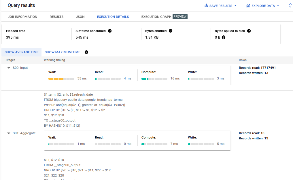
Instead, BigQuery records the query plan and timing information on every query job. If you run your queries in the BigQuery console, you can see them in the query's Execution details tab:
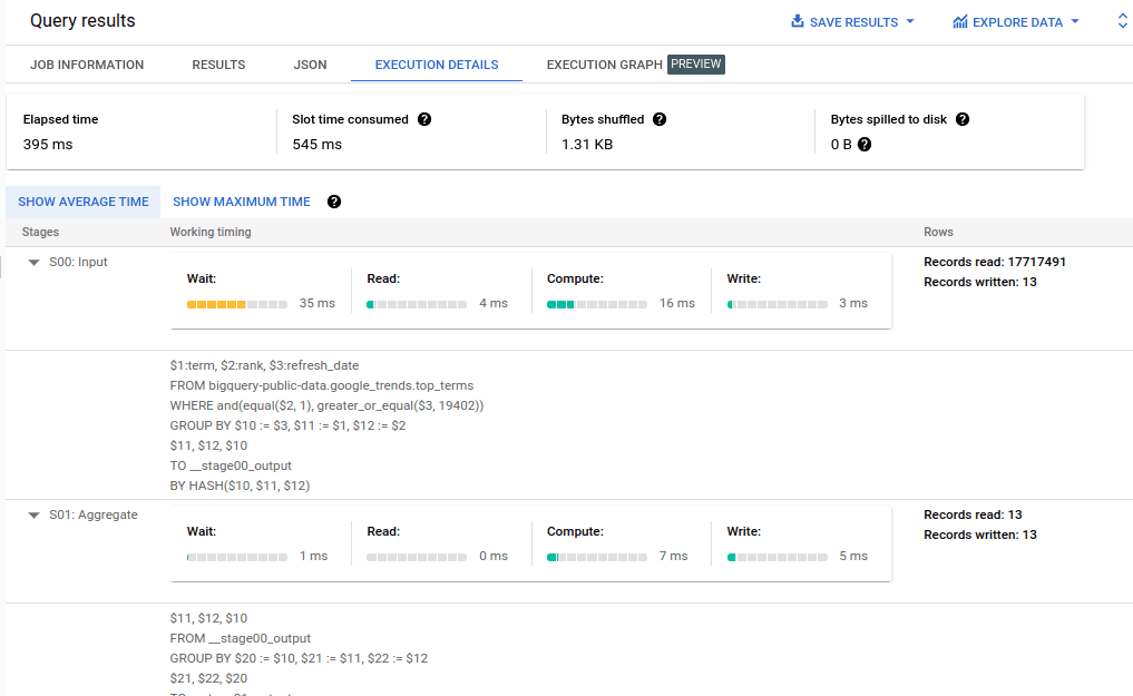 BigQuery does a pretty remarkable job here, processing 17,717,491 rows in under 395 milliseconds.
The query below returns the top search term in the US for each day of the last 2 weeks:
SELECT
   refresh_date AS Day,
   term AS Top_Term,
       -- These search terms are in the top 25 in the US each day.
   rank,
FROM `bigquery-public-data.google_trends.top_terms`
WHERE
   rank = 1
       -- Choose only the top term each day.
   AND refresh_date >= DATE_SUB(CURRENT_DATE(), INTERVAL 2 WEEK)
       -- Filter to the last 2 weeks.
GROUP BY Day, Top_Term, rank
ORDER BY Day DESC
   -- Show the days in reverse chronological order.
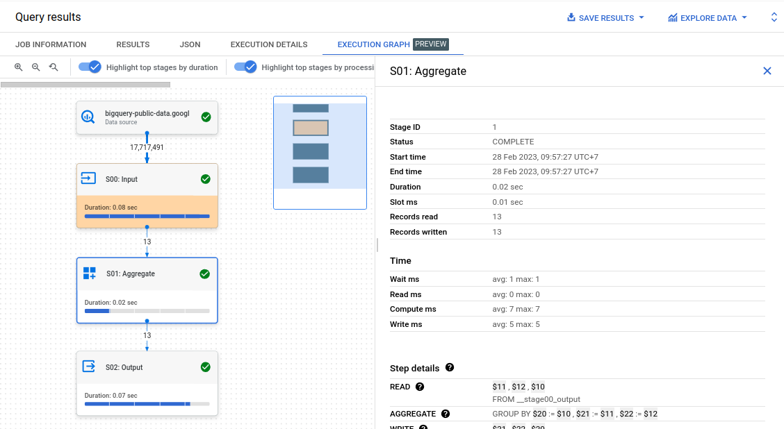
Since the most recent day has yet to conclude, we expect this query to return 13 rows. The details show an elapsed time of 395 milliseconds and how many bytes were processed. The Execution graph tab shows the query plan as a DAG (directed acyclic graph) of the stages BigQuery ran.
BigQuery breaks this query into 3 stages. It distributes the first two ("S00: Input" and "S01: Aggregate") across many workers that run in parallel, then combines their results in the last stage ("S02: Output"). Because the work is split up, some workers finish later than others. Toggling between "Show Average Time" and "Show Maximum Time" shows the gap between a typical worker and the slowest one in each stage.
In each stage, the execution details and the execution graph show how many records went in and how many came out.
-
In S00: Input, BigQuery reads 17,717,491 rows from
bigquery-public-data.google_trends.top_termsand applies theWHERE rank = 1 AND refresh_date >= ...filter, keeping only the 13 rows that match. Unsurprisingly, read and compute time are highest here. -
In S02: Output, BigQuery sorts the 13 rows for our
ORDER BYclause and returns them. This takes longer than the Aggregate stage, but is still much faster than Input.
When you read a BigQuery query plan, look out for:
- Bytes read per stage. The fewer bytes a stage processes, the faster it runs. This is part of why the Input stage is usually the longest.
- Bytes shuffled between stages. A large shuffle means a lot of data is moving between workers. If this is your bottleneck, check that the table is partitioned and clustered for the query.
- Records in vs records out. A stage that writes far more rows than it reads, or that passes millions of rows into a
JOINonly for most of them to be dropped later, is a sign you should filter or aggregate earlier. - Maximum time vs average time. A large gap means the work is unevenly spread, often because a few keys hold most of the data.
BigQuery also annotates the execution graph with query performance insights. A stage with an information icon has one, such as slot contention (not enough compute was available), insufficient shuffle quota, a join on non-unique keys that blew up the row count, or partition skew. Treat them as hints from BigQuery about where to look first.
If you're a developer, you can get the same information from the BigQuery client libraries. In Python, every query returns a QueryJob, which exposes the plan as query_plan and the bytes scanned as total_bytes_processed:
from google.cloud import bigquery

client = bigquery.Client()
sql = "SELECT term, rank FROM `bigquery-public-data.google_trends.top_terms` WHERE rank = 1"

# A dry run validates the query and reports how much it would scan, at no cost
dry = client.query(sql, job_config=bigquery.QueryJobConfig(dry_run=True, use_query_cache=False))
print(f"{dry.total_bytes_processed / 1e9:.2f} GB would be scanned")

job = client.query(sql)
job.result()
for stage in job.query_plan:
    print(stage.name, stage.records_read, stage.records_written, stage.slot_ms)
That dry run is the closest BigQuery gets to a plain EXPLAIN. It doesn't execute anything, it costs nothing, and it tells you how many bytes the query would process, which is what you pay for under on-demand pricing. The bq command line tool has the same option as bq query --dry_run, and the console runs one automatically as you type and shows the estimate in the editor.
To find which queries are worth optimizing in the first place, ask BigQuery for its job history. This lists the 10 queries that scanned the most data in the past week:
SELECT
  user_email,
  query,
  total_bytes_processed / POW(1024, 3) AS gb_processed,
  total_slot_ms
FROM `region-us`.INFORMATION_SCHEMA.JOBS_BY_PROJECT
WHERE creation_time > TIMESTAMP_SUB(CURRENT_TIMESTAMP(), INTERVAL 7 DAY)
  AND job_type = 'QUERY'
ORDER BY total_bytes_processed DESC
LIMIT 10;
What about the aforementioned Index scans?
BigQuery has no B-tree indexes, so there is no index scan in the Postgres sense. It stores each column separately and reads every value in each column a query touches, across every partition the query can't rule out. That's why SELECT * is the most expensive habit you can bring over from Postgres. On an unclustered table, adding LIMIT doesn't reduce the bytes read either.
The upside is that there is no index to design, maintain, or second-guess the planner about. The downside is that you lose some direct control: you can't add an index to rescue one slow query. Instead, BigQuery scales out. Queries run on slots (units of compute), and a query that needs more parallelism gets more of them, up to what your project has available.
For finding rows by value, such as looking up an order ID in a large log table, BigQuery offers search indexes:
CREATE SEARCH INDEX logs_index
ON my_dataset.app_logs(ALL COLUMNS);

SELECT event_time, message
FROM my_dataset.app_logs
WHERE SEARCH(app_logs, 'order-8812');
BigQuery maintains the index for you, and it can also speed up some =, IN and LIKE filters. It's the nearest thing BigQuery has to a Postgres index, and it's built for needle-in-a-haystack lookups rather than analytics over many rows.
Speeding up your queries with Clustered Tables and Partitioned Tables in BigQuery
For analytics queries, the main tools are partitioning and clustering. Suppose the data analysts on our team mostly query shipment status by date and country. We can create a table that is clustered by date and country to optimize for these queries.
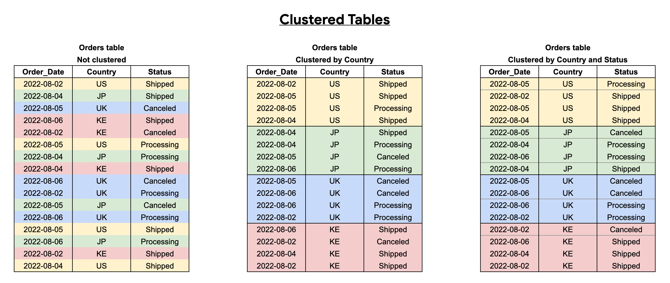
Clustering sorts the table's storage by those columns, so a query that filters on them can skip the blocks that can't match. Queries that filter on other columns won't benefit. A design decision like this is typically made by the data architects based on the queries the analysts and business users actually run. It's also why at Supertype we advocate for a full-cycle approach to building and scaling data architectures for our clients.
Running some benchmarks using the same query on a clustered table and an unclustered one, we get the same result with very different query times and costs.
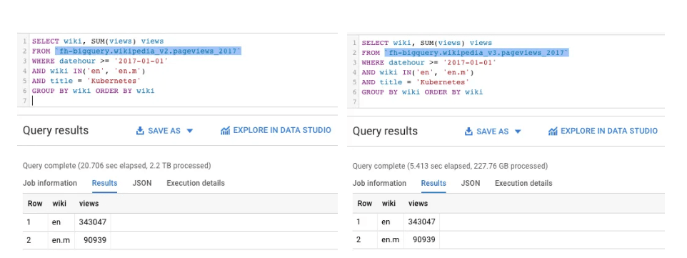
The query on the left processed 2.2 TB in 20.7 seconds, while the one on the right finished in 5.4 seconds at one-tenth of the cost.
Partitioning goes a step further. It splits a table into segments by a date, timestamp, or integer column, and a query that filters on that column reads only the partitions it needs. The two work together: BigQuery first skips the partitions outside your filter, then uses clustering to skip blocks within the partitions it does read.
CREATE TABLE shipments.status_daily
PARTITION BY ship_date
CLUSTER BY country, status
OPTIONS (require_partition_filter = TRUE)
AS SELECT * FROM shipments.status_raw;
require_partition_filter makes BigQuery reject any query on the table that doesn't filter on ship_date, so nobody scans the full history by accident. A table can have one partitioning column and up to four clustering columns, in order of how often you filter on them.
BigQuery query optimization checklist
Most BigQuery optimization comes down to reading less data and doing less work with it. Roughly in order of how often each one pays off:
- Select only the columns you need. Use
SELECT * EXCEPT (...)when you need nearly all of them. - Filter on the partitioning column in every query, and turn on
require_partition_filterfor large tables. - Cluster on the columns you filter and join on most, starting with the one you filter on most often.
- Filter and aggregate before a
JOIN, so fewer rows move between workers. - Put the largest table first in a join, then the smallest, then the rest by decreasing size.
- Join on
INT64keys rather than strings where you can. Wider keys take longer to compare. - Don't count on
WITHclauses for speed. BigQuery can evaluate a CTE each time it's referenced. Write an expensive intermediate result to a temporary table instead. - Use
ORDER BYonly in the outermost query, together withLIMIT. - Replace self joins with window functions.
- Use
APPROX_COUNT_DISTINCTinstead ofCOUNT(DISTINCT ...)when a close estimate is good enough, as it usually is on dashboards. - Precompute repeated aggregations with materialized views, which BigQuery keeps up to date as the base table changes.
- Add a search index for lookups by ID or keyword in large tables.
Postgres vs BigQuery: the optimization toolkit side by side
If you're migrating from Postgres to BigQuery, or moving data from BigQuery back into Postgres, it helps to know what replaces each familiar tool:
| What you want to do | PostgreSQL | BigQuery |
|---|---|---|
| See the plan before running | EXPLAIN | Dry run (bytes estimate) |
| See what actually ran | EXPLAIN ANALYZE | Execution details and execution graph |
| Skip rows you don't need | B-tree index | Partitioning and clustering |
| Find a row by value | B-tree index | Search index |
| Find your most expensive queries | pg_stat_statements | INFORMATION_SCHEMA.JOBS |
| Reuse expensive aggregations | Materialized view, refreshed manually | Materialized view, refreshed automatically |
| Throw more compute at it | A bigger server | More slots |
Closing: Overcoming performance bottlenecks on the database architectural layer
In our hypothetical scenario, we started our diagnosis at the bottom of the analytics stack: the database. Since we're in the middle of migrating from an on-premise PostgreSQL database to BigQuery, we looked at the tools each one gives us.
In Postgres, we read the plan with EXPLAIN ANALYZE and add indexes where the plan shows sequential scans on hot queries. In BigQuery, we use dry runs to check what a query will scan before running it, read the execution graph and its insights when it's slow, and design tables around partitioning and clustering so most queries read a fraction of the data.
In the next article in this series, we'll move up the stack to the "search" layer, and look at how we can further optimize our search queries so that our analysts can spend less time goofing around with "faux coffee breaks" in between waiting for their queries to finish, and more time analyzing the data.
Further reading
Like this piece? Take home The Enterprise AI Agentic Stack.
The same thinking runs all the way through this 12-chapter guide, written by Samuel Chan and ready to read in an afternoon.
Claude for Market Analysis
A hands-on workshop for building a personal market-monitoring system with Claude: screen IDX and SGX stocks, set up alerts in plain English, and build a live dashboard with an analyst built in. Beginner-friendly.
October 28, 2026Zoom Conferencing (Online)
Keep reading
Databases & BigQuery
Optimizing full text search in Postgres and BigQuery
A discussion on full text search and indexing strategies in Postgres and BigQuery (part 2 of 2)
Databases & BigQuery
Querying JSON data in Postgres
Filter rows on values inside a JSONB column with @>, ->> and ILIKE, and unpack nested arrays with jsonb_array_elements. Examples use real IDX company data.
Databases & BigQuery
Introduction to NoSQL
A general introduction to NoSQL databases and their use cases.
Field notes, straight to your inbox
We publish what we learn building analytics and AI systems for some of the largest enterprises in the region. Subscribe and we will send the next one your way.